Table Of Content

Next, the three dosage strengths are randomly assigned to split-plots. Finally, for each dosage strength, the capsules are created with different wall thicknesses, which is the split-split factor and then tested in random order. A split-plot design is a designed experiment that includes at least one hard-to-change factor that is difficult to completely randomize because of time or cost constraints.

Sorry, you have been blocked
The brownie example includes 2 whole plots replicated twice (total of 4 whole plots). The whole plot is all the trays of brownies being baked at the temperature. Thus, the ingredients act as the “whole” plot factors and other factors like temperature and baking time are used as the “split” plot factors. A split-plot design leads to an increase in precision in the estimates for all factor effects except for the whole-plot main effects. Split-level house plans can also incorporate multiple decks and balconies on the different floors.
Advantages of Split-Plot Designs
We have already seen that varying two factors simultaneously provides an effective experimental design for exploring the main (average) effects and interactions of the factors1. However, in practice, some factors may be more difficult to vary than others at the level of experimental units. For example, drugs given orally are difficult to administer to individual tissues, but observations on different tissues may be done by biopsy or autopsy. When the factors can be nested, it is more efficient to apply a difficult-to-change factor to the units at the top of the hierarchy and then apply the easier-to-change factor to a nested unit. (a) Basic time course design, in which time is one of the factors. (b) In a repeated measures design, mice are followed longitudinally.
Split-Level House Plans
You're going to use design of experiments to study 2 fertilizers and 4 seed varieties to see which combination provides the best crop yield. Using traditional design of experiments methods, you would randomly assign each fertilizer and seed combination to a different plot of land, eight plots in all. Each whole plot contains two subplots and fertilizer type is assigned to each subplot using RCBD (i.e. whole plots are treated as blocks and fertilizer type is assigned randomly within each whole plot to the subplots).
Multi-response optimization of Artemia hatching process using split-split-plot design based response surface ... - Nature.com
Multi-response optimization of Artemia hatching process using split-split-plot design based response surface ....
Posted: Mon, 16 Jan 2017 08:00:00 GMT [source]
Plan: #116-1091
The answer involves whether we are interested in specific levels of the factor or are using it for blocking purposes. In Figure 1b, the field is a blocking factor because it is used to control the variability of the plots, not as a systematic effect. In Figure 1c, irrigation is a whole plot factor and not a blocking factor because we are studying the specific levels of irrigation.
Statistics for Biologists
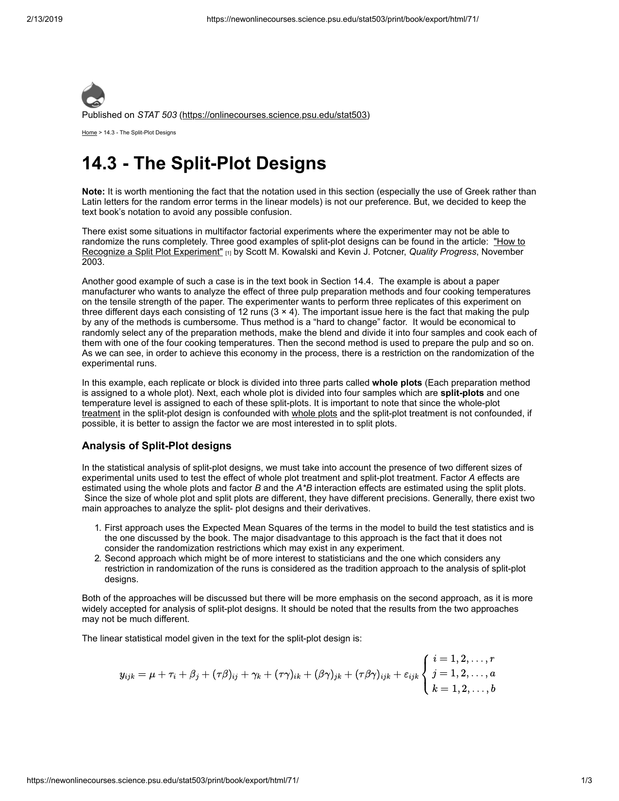
The important issue here is the fact that making the pulp by any of the methods is cumbersome. It would be economical to randomly select any of the preparation methods, make the blend and divide it into four samples and cook each of them with one of the four cooking temperatures. As we can see, in order to achieve this economy in the process, there is a restriction on the randomization of the experimental runs. They are experimenting with two levels of chocolate and sugar using two different baking temperatures. However, to save time they decide to bake more than one tray of brownies at the same time instead of baking each tray individually.
Understanding the factors controlling biofilm as an autochthonous resource in shaded oligotrophic neotropical streams
Figure 2 illustrates split plot designs in a biological context. If we only consider fertilization scheme, we do a completely randomized designhere, with plots as experimental units. The first part of model formula(7.1) is actually the corresponding model equation ofthe corresponding one-way ANOVA. Suppose that we wish to determine the in vivo effect of a drug on gene expression in two tissues. The mouse is the whole plot experimental unit and the drug is the whole plot factor. The tissue is the subplot factor and each mouse acts as a block for the tissue subplot factor; this is the RCBD component (Fig. 2a).
Plans Now License Agreement Preview
Now suppose varying the level of irrigation is difficult on a small scale and it makes more sense to apply irrigation levels to larger areas of land. To analyze the treatment effects we first follow the approach discussed in the book. Table 14.17 shows the expected mean squares used to construct test statistics for the case where replicates or blocks are random and whole plot treatments and split-plot treatments are fixed factors. Here, we can not simply randomize the 36 runs in a single block (or replicate) because we have our first hard to change factor, named Technician.
The split plot CRD design (Fig. 2a) is commonly used as the basis for a repeated measures design, which is a type of time course design. The most basic time course includes time as one of the factors in a two-factor design. In a completely randomized time course experiment, different mice are used at each of the measurement times t1, t2 and t3 after initial treatment (Fig. 3a). If the same mouse is used at each time and the mice are assigned at random to the levels of a (time-invariant) factor, the design becomes a repeated measures design (Fig. 3b) because the measurements are nested within mouse.
We can visualize the data with an interaction plot which shows that mass islarger on average with the new fertilization scheme. The interaction is not very pronounced (the variety effectseems to be consistent across the two fertilization schemes). If we consider the two treatment factors fertilizer and variety, the designlooks like a “classical” factorial design at first sight. In this scenario, the wood type is the hard-to-change factor “whole” plot factor and the temperature is the easy-to-change “split” plot factor. Both of the approaches will be discussed but there will be more emphasis on the second approach, as it is more widely accepted for analysis of split-plot designs. It should be noted that the results from the two approaches may not be much different.
GCMOnline.com - Golf Course Management magazine
GCMOnline.com.
Posted: Wed, 24 Apr 2024 13:30:19 GMT [source]
Applying blocking at the whole plot level, such as housing (Fig. 2b), can improve sensitivity for the whole plot factor similarly to using a RCBD. So far, we have not considered whether managing levels of irrigation and fertilizer require the same effort. If varying irrigation on a small scale is difficult, it makes more sense to irrigate larger areas of land than in Figure 1a and then vary the fertilizer accordingly to maintain a balanced design. If our land is divided into four fields (whole plots), each of which can be split into two subplots (Fig. 1c), we would assign irrigation to whole plots using CRD. Within a whole plot, fertilizer would be distributed across subplots using RCBD, randomly and balanced within whole plots with a given irrigation level.
To show how the analysis can be done for a split-plot design, we consider the case of equal sample sizes and randomized complete block designs for each of the treatment factors. There are then \(s\) blocks, each of which is divided into \(a\) whole plots, and each of these is subdivided into \(b\) split plots, giving a total of \(s a b\) observations. In a split-plot design with Factor A assigned to whole plots and Factor B assigned to split-plots, it is possible that there are no blocks for factor 1.
Frequently you will find living and dining areas on the main level with bedrooms located on an upper level. In Figure 7.1we can observe that blocks are different (this is why we use them), there is noclear effect of variety (V), but there seems to be a more or less lineareffect of nitrogen (N). The last statement produces 99% simultaneous confidence intervals for treatment-versus-control comparisons using Dunnett’s method. Compare the results with those provided in Sec 19.3 where step-by-step construction of the confidence intervals were shown. Blocks are quite often used in a split-plot design as illustrated by the following example. Statology is a site that makes learning statistics easy by explaining topics in simple and straightforward ways.
The lower level exits to the garage as well and usually has a rec room, a bedroom, and sometimes even a second kitchen which makes them a great alternative to the in-law suite or for older kids that have moved back home. Whether you do it through crop dusting or using one of the fancy new water-soluble fertilizers, you can apply fertilizer only to a large area. Split-plot designs were originally used in agriculture where the whole plots referred to a large area of land and the sub-plots were smaller areas within each whole plot. Split-plot designs are often used in manufacturing because there is often some variable that is produced in large quantities and thus it makes sense to carry out a split-plot design to reduce the cost of running an experiment.
Suppose there are \(a\ell\) whole plots where \(a\) is the number of levels of factor \(A\). Please note that test for equal effects for \(A\) requires the whole plot error as the denominator. The model is specified as we did earlier for the split-plot in RCBD, retaining only the interactions involving replication where they form denominators for \(F\)-tests for factor effects. For the model above, we would need to include the block, block × A, and block × A × B terms in the random statement in SAS. In SAS, Block × A × B would automatically include the Block × B effect SS and df.
Again, there is no free lunch,this is the price that we pay for the “laziness.” More information can forexample be found in Goos, Langhans, and Vandebroek (2006). A wood manufacturer wants to find the optimal mix of wood type and temperature to produce the most durable wood. Since the type of wood can take a long time to acquire, they may apply three different temperatures to two different wood types. In this particular example, it’s not possible to apply different irrigation methods to areas smaller than one field, but it is possible to apply different fertilizers to small areas. This type of design was developed in 1925 by mathematician Ronald Fisher for use in agricultural experiments. Split level homes offer living space on multiple levels separated by short flights of stairs up or down.


No comments:
Post a Comment